3.1. Annealing the posterior distribution

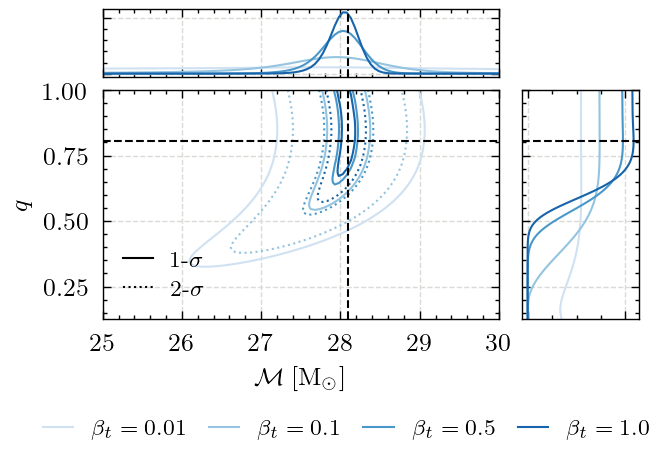
This notebooks includes code to produce Figure 2 in the paper. This shows how the evolution of the annealed posterior distribution

\[ p(\theta|d, \beta_t) = \frac{p(d|\theta)^{\beta_t}p(\theta)}{p(d)}, \]

as a function of \(\beta_t\).

We use bilby to define the likelihood and prior based on the examples include in the bibly repository.

Imports

Import the modules we’re going to use and set the plotting style for consistency with other figures.

import bilby
import matplotlib.pyplot as plt
from matplotlib.lines import Line2D
import multiprocessing as mp
import numpy as np
import os
import pandas as pd
import pathlib
import seaborn as sns
import warnings

from gw_smc_utils.plotting import set_style

warnings.filterwarnings("ignore", "Wswiglal-redir-stdio")
import lal  # noqa: E402

# Suppress lal's redirection of standard output and error
lal.swig_redirect_standard_output_error(False)

# Set the number of threads for OpenMP to 1 to avoid issues with parallelization
os.environ["OMP_NUM_THREADS"] = "1"

set_style()

General configuration

Define the output directory for the figure and ensure it exists

figure_dir = pathlib.Path("figures")
figure_dir.mkdir(exist_ok=True)

Configure the bilby logger to only print warnings.

bilby.core.utils.setup_logger(log_level="WARNING")

Data and Injection configuration

Define the duration of the data, sampling frequency and minimum frequency.

duration = 4.0
sampling_frequency = 2048.0
minimum_frequency = 20

Define a GW150914-like injection and generate all the derived parameters.

injection_parameters = dict(
    mass_1=36.0,
    mass_2=29.0,
    a_1=0.4,
    a_2=0.3,
    tilt_1=0.5,
    tilt_2=1.0,
    phi_12=1.7,
    phi_jl=0.3,
    luminosity_distance=3000.0,
    theta_jn=0.4,
    psi=2.659,
    phase=1.3,
    geocent_time=1126259642.413,
    ra=1.375,
    dec=-1.2108,
)
injection_parameters = bilby.gw.conversion.generate_all_bbh_parameters(
    injection_parameters
)

Likelihood and priors

We then construct the likelihood and prior objects.

We define a waveform generator using IMRPhenomPv2 and two-detector network with H1 and L1. We then inject the GW150914-like signal.

We then construct the prior dictionary and fix all the parameters, except for the mass parameters and phase.

For the likelihood, we use the standard GravitationalWaveTransient class from bilby and enable phase marginalization.

waveform_arguments = dict(
    waveform_approximant="IMRPhenomPv2",
    reference_frequency=50.0,
    minimum_frequency=minimum_frequency,
)

waveform_generator = bilby.gw.WaveformGenerator(
    duration=duration,
    sampling_frequency=sampling_frequency,
    frequency_domain_source_model=bilby.gw.source.lal_binary_black_hole,
    parameter_conversion=bilby.gw.conversion.convert_to_lal_binary_black_hole_parameters,
    waveform_arguments=waveform_arguments,
)

ifos = bilby.gw.detector.InterferometerList(["H1", "L1"])
ifos.set_strain_data_from_zero_noise(
    sampling_frequency=sampling_frequency,
    duration=duration,
    start_time=injection_parameters["geocent_time"] - 2,
)
ifos.inject_signal(
    waveform_generator=waveform_generator, parameters=injection_parameters
)

priors = bilby.gw.prior.BBHPriorDict()
for key in [
    "a_1",
    "a_2",
    "tilt_1",
    "tilt_2",
    "phi_12",
    "phi_jl",
    "psi",
    "ra",
    "dec",
    "geocent_time",
    "luminosity_distance",
    "theta_jn",
]:
    priors[key] = injection_parameters[key]

priors.validate_prior(duration, minimum_frequency)

priors["chirp_mass"] = bilby.core.prior.Uniform(25, 30)
priors["mass_ratio"] = bilby.core.prior.Uniform(0.125, 1)
priors.pop("mass_1")
priors.pop("mass_2")

likelihood = bilby.gw.GravitationalWaveTransient(
    interferometers=ifos,
    waveform_generator=waveform_generator,
    priors=priors,
    phase_marginalization=True,
)

Parameter grid

We then define a grid in mass ratio and chirp mass over which we will evaluate the log-likelihood and log-prior.

We parallelize the likelihood calculation to speed things up. This requires use to define a helper function log_likelihood so we can use pool.map.

# Define grid
n = 100
chirp_mass_vec = np.linspace(
    priors["chirp_mass"].minimum, priors["chirp_mass"].maximum, n
)
mass_ratio_vec = np.linspace(
    priors["mass_ratio"].minimum, priors["mass_ratio"].maximum, n
)
chirp_mass, mass_ratio = np.meshgrid(chirp_mass_vec, mass_ratio_vec)
chirp_mass = chirp_mass.flatten()
mass_ratio = mass_ratio.flatten()

# Create theta dictionary for the grid, this ensure any additional parameters are included
theta = priors.sample(len(chirp_mass))
theta["chirp_mass"] = chirp_mass
theta["mass_ratio"] = mass_ratio
theta_df = pd.DataFrame(theta)
theta_list = theta_df.to_dict(orient="records")


# Function to compute log likelihood for a given theta
def log_likelihood(theta):
    likelihood.parameters.update(theta)
    return likelihood.log_likelihood()


# Use multiprocessing to compute log likelihoods in parallel
with mp.Pool(processes=4) as pool:
    logl = np.array(pool.map(log_likelihood, theta_list))

logp = priors.ln_prob(theta, axis=0)

14:55 bilby WARNING : Prior sampling efficiency is very low, please verify its validity.

Posterior weights

We then compute the unnormalized posterior weights for four different inverse temperatures (beta)

betas = np.array([1e-2, 1e-1, 0.5, 1.0])

weights = []
for beta in betas:
    logw = beta * logl + logp
    logw -= np.max(logw)
    w = np.exp(logw)
    weights.append(w)

weights = np.array(weights)

Figure 2 - Annealed posterior distribution

With this, we have everything we need to produce the figure.

fig = plt.figure()
gs = fig.add_gridspec(4, 4)
ax_joint = fig.add_subplot(gs[1:4, 0:3])
ax_marg_x = fig.add_subplot(gs[0, 0:3], sharex=ax_joint)
ax_marg_y = fig.add_subplot(gs[1:4, 3], sharey=ax_joint)

linestyles = [":", "-"]
colours = sns.color_palette("Blues", len(betas))

legend_handles = []

for beta, w, c in zip(betas, weights, colours):
    # ax.scatter(theta["chirp_mass"], theta["mass_ratio"], c=w)

    mass_ratio_grid = mass_ratio.reshape(n, n)
    chirp_mass_grid = chirp_mass.reshape(n, n)
    w_grid = w.reshape(n, n)

    n_levels = 2
    cc = n_levels * [c]
    ax_joint.contour(
        chirp_mass_grid,
        mass_ratio_grid,
        w_grid,
        levels=(1 - np.exp(-0.5), 1 - np.exp(-2)),
        colors=cc,
        linestyles=linestyles,
        negative_linestyles="-.",
    )

    # Compute marginal distributions by summing over the other parameter
    # and normalizing such that the sum is 1.
    marg_chirp_mass = np.sum(w_grid, axis=0)
    marg_mass_ratio = np.sum(w_grid, axis=1)
    marg_chirp_mass /= np.sum(marg_chirp_mass)
    marg_mass_ratio /= np.sum(marg_mass_ratio)

    ax_marg_x.plot(chirp_mass_grid[0, :], marg_chirp_mass, color=c)
    ax_marg_y.plot(marg_mass_ratio, mass_ratio_grid[:, 0], color=c)

    legend_handles.append(
        Line2D(
            [0],
            [0],
            color=c,
            linestyle="-",
            label=r"$\beta_t={}$".format(beta),
        )
    )

# Disable tick labels on marginal axes
ax_marg_x.tick_params(labelbottom=False)
ax_marg_x.tick_params(labelleft=False)
ax_marg_y.tick_params(labelleft=False)
ax_marg_y.tick_params(labelbottom=False)

ax_joint.set_xlabel(r"$\mathcal{M} \;[{\rm M}_{\odot}]$")
ax_joint.set_ylabel(r"$q$")


# Add injection parameters as dashed lines
ax_joint.axvline(
    injection_parameters["chirp_mass"],
    color="k",
    linestyle="--",
)
ax_joint.axhline(
    injection_parameters["mass_ratio"],
    color="k",
    linestyle="--",
)

ax_marg_x.axvline(
    injection_parameters["chirp_mass"],
    color="k",
    linestyle="--",
)

ax_marg_y.axhline(
    injection_parameters["mass_ratio"],
    color="k",
    linestyle="--",
)


fig.legend(
    handles=legend_handles,
    loc="upper center",
    bbox_to_anchor=(0.5, -0.025),
    ncol=4,
)

ax_joint.legend(
    handles=[
        Line2D([0], [0], color="k", linestyle="-", label="1-$\sigma$"),
        Line2D([0], [0], color="k", linestyle=":", label="2-$\sigma$"),
    ]
)

plt.show()
fig.savefig(figure_dir / "chirp_mass_mass_ratio_temperature.pdf", bbox_inches="tight")