3.2. Evolution of a run with pocomc

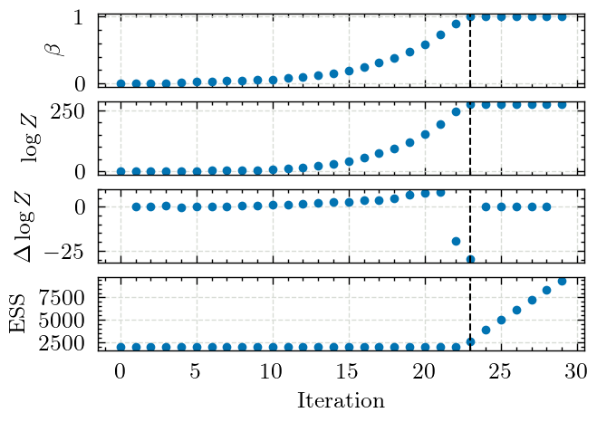
This notebooks includes code to produce Figure 3 in the paper. This shows how the inverse temperature, log-evidence and effective sample size evolve throughout a run using pocomc to analyse GW150914.

Imports

Import various modules, set the plotting style and the output directory for the figures.

import matplotlib.pyplot as plt
import numpy as np
import pickle
from pathlib import Path

from gw_smc_utils.plotting import set_style

set_style()

figure_dir = Path("figures")
figure_dir.mkdir(exist_ok=True)

Data release path

Define the path to the state file from the pocomc run.

We use one of the parallel runs from the analysis of GW150914 that described later in the paper.

data_release_path = Path("../data_release/gw_smc_data_release_core/")
state_file = data_release_path / "real_data" / "GW150914_pocomc_final_state.state"

Loading the pocomc checkpoint file

Load the state file using pickle and get the relevant quantities.

For further details, see the pocomc documentation.

with open(state_file, "rb") as f:
    state = pickle.load(f)

particles = state["particles"]
beta = particles.get("beta")
ess = particles.get("ess")
log_z = particles.get("logz")

Producing Figure 3

Plot the statistics as as function of iteration

figsize = plt.rcParams["figure.figsize"].copy()
figsize[1] *= 1.2
fig, axs = plt.subplots(4, 1, sharex=True, figsize=figsize)

axs[0].plot(beta, ls="", marker=".")
axs[0].set_ylabel(r"$\beta$")

axs[1].plot(log_z, ls="", marker=".")
axs[1].set_ylabel(r"$\log Z$")

axs[2].plot(
    np.arange(1, len(beta) - 1), np.diff(log_z[1:] - log_z[:-1]), ls="", marker="."
)
axs[2].set_ylabel(r"$\Delta\log Z$")

axs[3].plot(ess, ls="", marker=".")
axs[3].set_ylabel("ESS")

final_smc_it = np.argmax(beta == 1)

# Add vertical lines to indicate the final SMC iteration when beta reaches 1
for ax in axs:
    ax.axvline(final_smc_it, color="black", linestyle="--")

axs[-1].set_xlabel("Iteration")
fig.savefig(figure_dir / "pocomc_history.pdf")