Jensen-Shannon Divergence

This notebook contains code to reproduce Figure 5 from the paper. It uses precomputed Jensen-Shannon divergences which are included in the data release.

Imports

import matplotlib.pyplot as plt
from matplotlib.patches import Patch
from matplotlib.backends.backend_pgf import FigureCanvasPgf
import numpy as np
import seaborn as sns
import json
from pathlib import Path
import pandas as pd
import glob
from natsort import natsorted
import os
import re

from pesummary.gw.plots.latex_labels import GWlatex_labels

from gw_smc_utils.plotting import set_style

GWlatex_labels["azimuth"] = r"$\epsilon$"
GWlatex_labels["zenith"] = r"$\kappa$"

set_style()

Data release path

We specify the path to the data release and to the injection file.

data_release_path = Path("../data_release/gw_smc_data_release_core")

injections = pd.read_hdf(
    data_release_path / "simulated_data" / "pp_tests" / "pp_test_injection_file.hdf5",
    "injections",
)

Loading the JSD values

We define a function to load the JSD values from the files in the data release

def load_values(path, key="jsd"):
    files = natsorted(glob.glob(os.path.join(path, "*.json")))
    values = []
    for fd in files:
        with open(fd, "r") as f:
            entry = json.load(f)
        values.append({k: np.median(v) for k, v in entry[key].items()})
    df = pd.DataFrame(values)
    return df

Specify the path to the JSD results

jsd_path = data_release_path / "simulated_data" / "pp_tests" / "jsd_results"
jsd_path_2det = jsd_path / "2det"
jsd_path_3det = jsd_path / "3det"

We check for missing results

# Check for missing JSD results
n_injections = len(injections)
for p in [jsd_path_2det, jsd_path_3det]:
    missing = []
    for i in range(n_injections):
        if not os.path.exists(p / f"data{i}.json"):
            missing.append(i)
    print(f"Missing JSD for {p}: {missing}")

Missing JSD for ../data_release/gw_smc_data_release_core/simulated_data/pp_tests/jsd_results/2det: []
Missing JSD for ../data_release/gw_smc_data_release_core/simulated_data/pp_tests/jsd_results/3det: []

Load JSD values.

Since we use the time of arrival at the detector with highest SNR when performing inference, we combine the JSD values for these into a single time variable.

jsds_2det = load_values(jsd_path_2det)
# Merge the time parameters into one
jsds_2det["time"] = jsds_2det["L1_time"].fillna(jsds_2det["H1_time"])

jsds_3det = load_values(jsd_path_3det)
# Merge the time parameters into one
jsds_3det["time"] = (
    jsds_3det["L1_time"].fillna(jsds_3det["H1_time"]).fillna(jsds_3det["V1_time"])
)

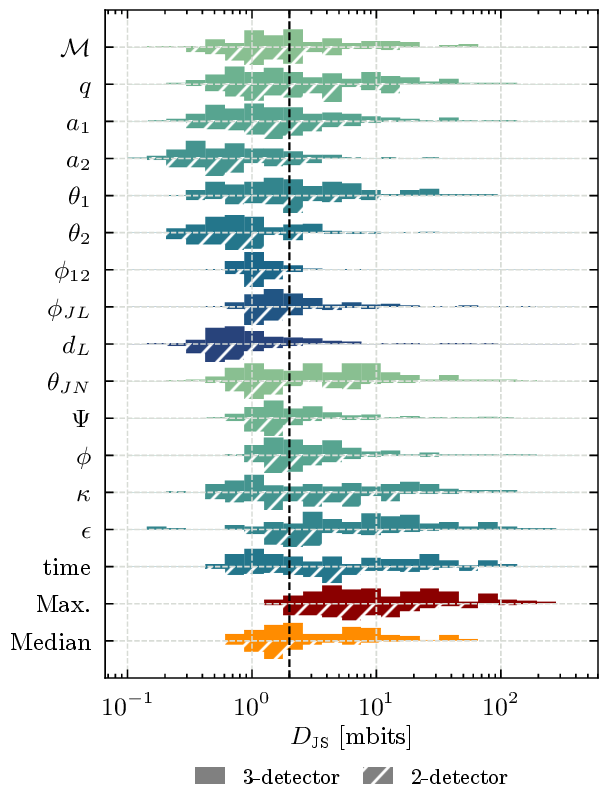
Figure 5 - JSD distributions

The code below produces the figure.

The figure is rasterized due to issues with rendering the hatching in PDFs.

top_df = jsds_3det
bottom_df = jsds_2det

left_label = "3-detector"
right_label = "2-detector"

label = "jsd_vertical"

n_bins = 24

sep = 2.1

single_width = sep / 2

# Get the list of parameters
parameters = jsds_3det.columns.tolist()
# Remove the per-detector times
parameters.remove("H1_time")
parameters.remove("L1_time")
parameters.remove("V1_time")
n_parameters = len(parameters)

max_jsd_top = np.array(top_df.T.max())
max_jsd_bottom = np.array(bottom_df.T.max())

median_jsd_left = np.array(top_df.T.mean())
median_jsd_right = np.array(bottom_df.T.median())


# Convert to mbits
base_conversion = 1000  # / np.log2

yticks = np.arange(0, (n_parameters + 2) * sep, sep)

left = 0

bins = np.logspace(-1, 2.6, n_bins, base=10)
factor = 1 * base_conversion

n_samples = 5000
threshold = (10 / n_samples) * 1000

colours = np.tile(sns.color_palette("crest", n_colors=9), (2, 1))

# For some reason, the this doesn't work in a context manager
plt.rcParams["hatch.linewidth"] = 1.0
with plt.rc_context(
    {
        "hatch.color": "white",
    }
):
    figsize = plt.rcParams["figure.figsize"].copy()
    figsize[0] = 1 * figsize[0]
    figsize[1] = 2 * figsize[1]
    fig = plt.figure(figsize=figsize)

    for i, parameter in enumerate(parameters):
        vals = top_df[parameter] * factor
        # print(vals)
        freqs, bin_edges = np.histogram(vals, bins=bins)
        freqs = freqs / freqs.max()
        bin_centres = (bin_edges[:-1] + bin_edges[1:]) / 2
        widths = np.diff(bin_edges)
        plt.bar(bin_centres, -freqs, bottom=left, width=widths, color=colours[i])

        vals = bottom_df[parameter] * factor
        # print(vals)
        freqs, bin_edges = np.histogram(vals, bins=bins)
        freqs = freqs / freqs.max()
        bin_centres = (bin_edges[:-1] + bin_edges[1:]) / 2
        widths = np.diff(bin_edges)
        plt.bar(
            bin_centres,
            freqs,
            bottom=left,
            width=widths,
            color=colours[i],
            hatch="///",
            # edgecolor=colours[i],
            rasterized=True,
        )

        left += sep

    freqs, bin_edges = np.histogram(max_jsd_top * factor, bins=bins)
    freqs = freqs / freqs.max()
    bin_centres = (bin_edges[:-1] + bin_edges[1:]) / 2
    widths = np.diff(bin_edges)
    plt.bar(
        bin_centres, -freqs, bottom=left, width=widths, color="darkred", rasterized=True
    )

    freqs, bin_edges = np.histogram(max_jsd_bottom * factor, bins=bins)
    freqs = freqs / freqs.max()
    bin_centres = (bin_edges[:-1] + bin_edges[1:]) / 2
    widths = np.diff(bin_edges)
    plt.bar(
        bin_centres,
        freqs,
        bottom=left,
        width=widths,
        color="darkred",
        hatch="///",
        rasterized=True,
    )

    left += sep

    freqs, bin_edges = np.histogram(median_jsd_left * factor, bins=bins)
    freqs = freqs / freqs.max()
    bin_centres = (bin_edges[:-1] + bin_edges[1:]) / 2
    widths = np.diff(bin_edges)
    plt.bar(
        bin_centres,
        -freqs,
        bottom=left,
        width=widths,
        color="darkorange",
        rasterized=True,
    )

    freqs, bin_edges = np.histogram(median_jsd_right * factor, bins=bins)
    freqs = freqs / freqs.max()
    bin_centres = (bin_edges[:-1] + bin_edges[1:]) / 2
    widths = np.diff(bin_edges)
    plt.bar(
        bin_centres,
        freqs,
        bottom=left,
        width=widths,
        color="darkorange",
        hatch="///",
        rasterized=True,
    )

    plt.xscale("log")
    plt.ylim(bottom=-sep, top=left + sep)

    plt.axvline(threshold, ls="--", color="k")

    ytick_labels = [
        GWlatex_labels.get(parameter, parameter) for parameter in parameters
    ]
    ytick_labels.append("Max.")
    ytick_labels.append("Median")
    # Remove units in square brackets
    ytick_labels = [re.sub(r"\[.*?\]", "", label) for label in ytick_labels]

    plt.yticks(
        yticks,
        labels=ytick_labels,
    )
    plt.tick_params(axis="y", which="minor", left=False, right=False)

    plt.gca().invert_yaxis()

    plt.xlabel(r"$D_{\rm JS}$ [mbits]")

    handles = [
        Patch(facecolor="grey", label=left_label),
        Patch(facecolor="grey", label=right_label, hatch="///"),
    ]

    plt.tight_layout()
    legend = plt.legend(
        handles=handles, loc="center", bbox_to_anchor=(0.5, -0.15), ncol=2
    )

    for patch in legend.get_patches():
        patch.set_rasterized(True)

    canvas = FigureCanvasPgf(fig)
    canvas.print_figure(f"figures/{label}.pdf", dpi=300)